Heart Beat

Medium

canvas

animation

motion

parametric

Animate a beating heart by plotting a parametric curve and scaling it rhythmically over time.

Goal

Render a heart using a parametric curve and animate it so it beats over time. The heart should stay centered on the canvas while its scale changes rhythmically. Your task is to implement the curve equation and the pulse scaling function, then draw the final polygon each frame.

JavaScript

Preview • sandboxed

Console output

The Beauty of Mathematics

Mathematics is often called the queen of sciences, and for good reason. With mathematical models and formulas, you can describe almost anything. In this task, we will see how mathematics can be used to describe the shape of a heart, and then try to bring it to life by recreating a heartbeat. ❤️

Heart Shape

There are many ways to describe a heart. The formulas differ slightly, and those differences affect the final shape. For example, you can define it in the classic implicit form:

(x^2+y^2-1)^3 - x^2y^3=0

Or in polar coordinates:

t = 1 - sin(\theta)

For easier implementation, it is more convenient to use a parametric formula. For example, one of the most common versions is:

x(p) = 2 cos(p) - cos(2p)

y(p) = 2 sin(p) - sin(2p)

But for this task, it is better to use one of the most elegant parametric forms:

x(p)=16sin^3(p)

y(p)=13cos(p) - 5 cos(2p) - 2 cos(3p) - cos(4p)

Where p lies in the interval [0,2π].

All these formulas are derived manually by transforming basic functions and fitting them to the desired shape. Unfortunately, there is no strict proof for why one of these forms describes a heart better or worse than another, so we will not go into that here.

Heartbeat

The heartbeat is created by scaling the shape. In other words, for each point of the heart (x, y), we define a scale factor beat(t), and get new coordinates (beat(t) * x, beat(t) * y). So how do we define beat(t)?

There is room for experimentation here as well. The most important thing is that the heartbeat function must be periodic, meaning it repeats its values over a fixed interval of time. For example, you could use a sinus function. But if we want behavior closer to a real heart, it is better to use a function like this:

Here, x is the normalized amount of time that has passed within a single period:

x(t) = (t \% period) / period

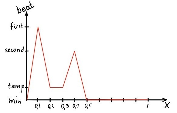
The function itself is piecewise-defined. That means we manually specify that first there is a linear rise and fall (the first heartbeat), then a short pause at an temp value, then a second linear rise and fall to the minimum value (the second heartbeat), and finally a long pause. So the behavior is close to reality: a beat, a smaller beat, then a pause. The values first, temp, second, and min are chosen manually.

To determine how beat(t) is defined on each segment, we can use the known intermediate values. For example, on the interval (0.1, 0.2], we know that at the point 0.1 the value is first, and at the point 0.2 the value is temp. We also know that beat function on this interval is linear, that is:

beat(x) = ax + b

We can substitute the endpoint values and obtain a system of linear equations:

first = a \cdot 0.1 + b

temp = a \cdot 0.2 + b

From this, we find the coefficients a and b, which gives us the following formula for the interval (0.1, 0.2]:

beat(t) = 10 \cdot (temp-first) \cdot x + 2 \cdot first - temp

Task: perform the same calculations for all intervals of the period.

Summary

Now you know how to define a mathematical heart shape and how to simulate its beating using scaling. Complete the task above and implement this game.

Walkthrough

The Beauty of Mathematics

Heart Shape

Heartbeat

Summary